About this demo
How we built this map (high-level)
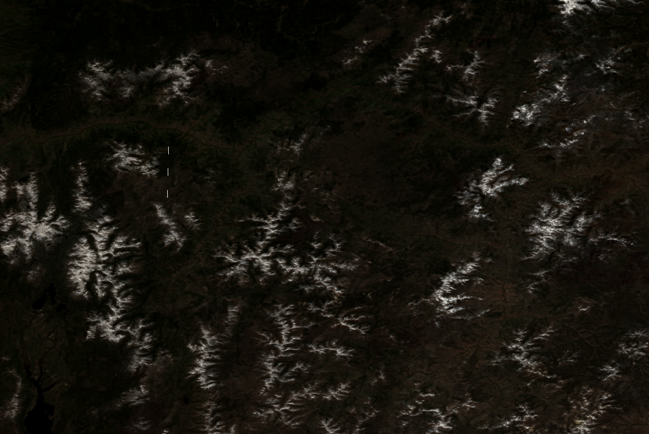
This surface layer blends multispectral satellite cues with network + tabular signals. Vision inputs included Sentinel‑2 RGB (B04,B03,B02), near‑infrared B08, and an NDVI composite (Q2 2025), along with NAIP RGB in select regions. We combine these with traffic & activity‑change indicators, elevation, land‑cover, proximity, and other engineered features in a set of latest‑generation vision transformers, ResNet‑style backbones, and tabular models, aggregated via ensembles to maximize stability. In total, the system fuses 18+ billion individual data points.
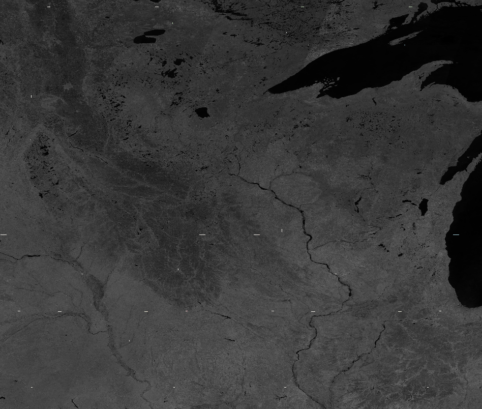
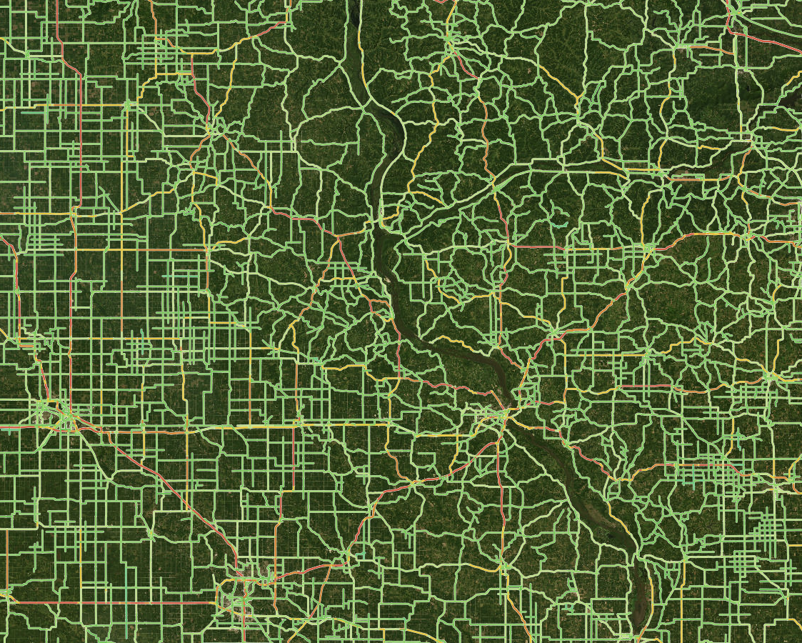
We also developed an experimental routing engine that can evaluate ~1 billion shortest paths per hour. Using global nighttime‑lights (e.g., VIIRS‑class sensors) as a proxy for population intensity, we sample OD pairs and accumulate a homogeneous traffic prior. This synthesized layer is one of many signals the model sees—helping it reason about where paved vs. unpaved is most likely, alongside terrain, land cover, and contextual features.
NDVI example (below): computed per‑pixel as
(NIR − Red) / (NIR + Red) from Sentinel‑2 B08 (near‑infrared) and B04 (red).
Values near 1.0 indicate healthy, dense vegetation; values near 0 often correspond to
bare soil, roads, or urban surfaces; negative values can indicate water or deep shadows. We colorize NDVI for
readability (higher NDVI appears greener), and use it as a stable seasonal cue to help separate paved vs.
unpaved in vegetated landscapes and to improve robustness under changing illumination.
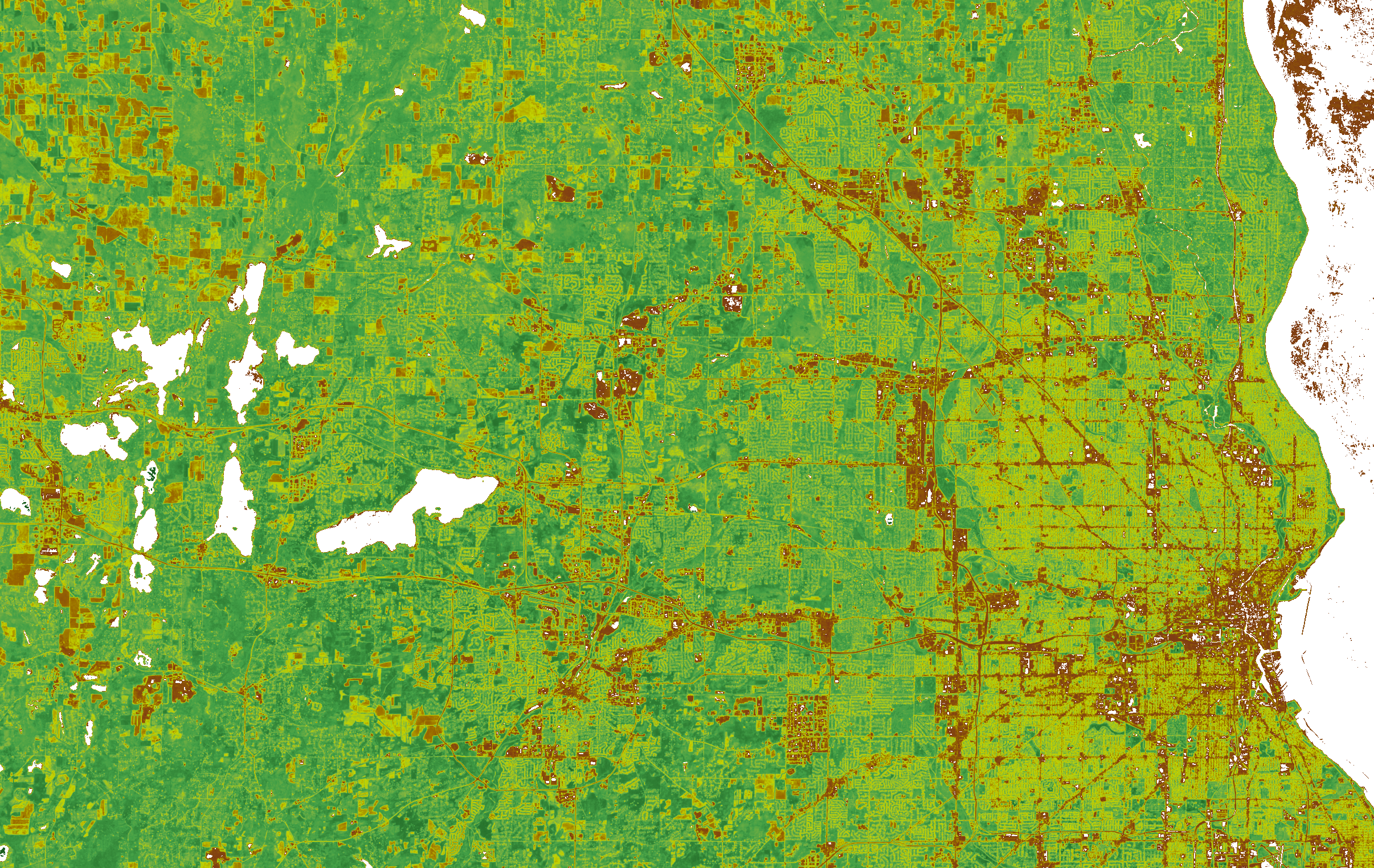
(NIR − Red) / (NIR + Red).
Higher values (greener) imply more vigorous vegetation; lower values (neutral/brown) are sparse vegetation,
soil, or roads. Click to view full‑resolution.
Notes: The background imagery you see in the map is for context; the classification can be more current than that imagery. Methods are proprietary and summarized here at a high level.
© Sherpa LLC — All rights reserved.